<?xml version="1.0" encoding="utf-8"?><feed xmlns="http://www.w3.org/2005/Atom" ><generator uri="https://jekyllrb.com/" version="3.10.0">Jekyll</generator><link href="machinesight.github.io/feed.xml" rel="self" type="application/atom+xml" /><link href="machinesight.github.io/" rel="alternate" type="text/html" /><updated>2026-05-10T13:59:19+00:00</updated><id>machinesight.github.io/feed.xml</id><title type="html">MachineSight</title><subtitle>Welcome to MachineSight. Here you will find insights, and tutorials on computer vision techniques.</subtitle><entry><title type="html">A Comprehensive Guide into Object Detection with Ultralytics YOLO</title><link href="machinesight.github.io/posts/a-comprehensive-guide-into-object-detection-with-ultralytics-yolo" rel="alternate" type="text/html" title="A Comprehensive Guide into Object Detection with Ultralytics YOLO" /><published>2026-04-25T11:30:55+00:00</published><updated>2026-04-25T11:30:55+00:00</updated><id>machinesight.github.io/posts/a-comprehensive-guide-into-object-detection-with-ultralytics-yolo</id><content type="html" xml:base="machinesight.github.io/posts/a-comprehensive-guide-into-object-detection-with-ultralytics-yolo"><![CDATA[<p><img src="/assets/images/2026-04-25/intro_img.png" alt="pothole, speedbump, and crack detection." /></p>
<figcaption>
 Pothole, speedbump, and crack detection.
</figcaption>
<p><br /></p>

<p>
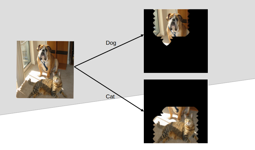
Object detection entails two major things: classification and localization. Classification answers “what object is there?” while localization answers “where is it?”. YOLO models have been excellent answering both questions at once, that is, they simultaneously classify objects in a scene and identify their particular location with bounding boxes.</p>

<p>
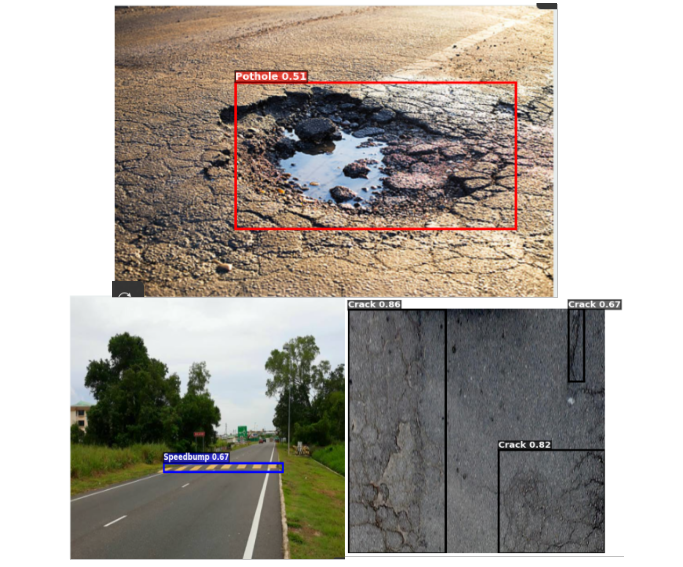
This blog post based on a class project, won’t go into the mathematical foundation of the YOLO algorithm but would rather walk through the process, typical of training and deploying an object detection model with Ultralytics-managed YOLO. We will train YOLO to detect three different kinds of road anomaly (crack, pothole, and speedbump) using publicly available datasets.</p>

<p><em>By the way, YOLO stands for You Only Look Once. See the <a href="https://arxiv.org/abs/1506.02640" target="_blank">paper</a> that introduced it for reference.</em></p>

<p>The usual pipeline has three main stages: <strong>Image Data Acquisition and Processing, Model Training, and Performance Evaluation and Testing</strong>. For the sake of large downloads, processing and ease of access, we will perform the first stage (image acquisition and processing) on our PC. However, the model training will take place on Kaggle because of the free accelerators (GPU) quota they provide, open an account at <a href="https://www.kaggle.com" target="_blank">kaggle.com</a> if you don’t have one. Then the cleaned dataset will be uploaded to Kaggle for the training. You may want to skip through to training, for this, access the cleaned dataset <a href="https://www.kaggle.com/datasets/david2do/road-anomaly-ds" target="_blank">here.</a></p>

<h3> Image Data Acquisition And Processing </h3>

<p>This is the most messy part of the process as lots of temporary files will be created and care needs to be taken to avoid painful errors. Again, you may want to skip through to training, for this, download the already prepared dataset at <a href="https://www.kaggle.com/datasets/david2do/road-anomaly-ds" target="_blank">Kaggle.</a></p>

<p>Because this is done locally on our PC, there are installations to make.
First, install a recent version of Python from the official release page at python.org. Once installed, make a directory and create a virtual environment by running this command</p>

<p><code class="language-plaintext highlighter-rouge">mkdir road-anomaly-ds &amp;&amp; cd road-anomaly-ds</code></p>

<p><code class="language-plaintext highlighter-rouge">python3 -m venv .road-anomaly-env</code></p>

<p>Activate the virtual environment created with</p>

<p><code class="language-plaintext highlighter-rouge">source .road-anomaly-env/bin/activate</code></p>

<p>Then we install numpy, matplotlib, and jupyter running</p>

<p><code class="language-plaintext highlighter-rouge">pip install numpy matplotlib jupyter</code></p>

<p>Now, we can download the raw datasets for each three classes via the following links:</p>

<blockquote>
  <p><a href="https://www.kaggle.com/datasets/rajdalsaniya/pothole-detection-dataset" target="_blank">Pothole</a> <br />
<a href="https://universe.roboflow.com/pothole-detection-1nczj/speed-unmarked-bumb" target="_blank">Speedbump</a> <br />
<a href="https://drive.google.com/drive/folders/1a1e-cTXoQpmzEXd4Uj4z9mAPJnmRGUbd" target="_blank">Crack</a></p>
</blockquote>

<p>Rename the downloaded folders accordingly and move them into the project directory road-anomaly-ds we created earlier.</p>

<p><strong>Overview of the datasets</strong></p>

<p>
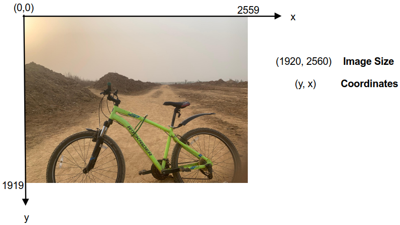
There are two most important parts to each dataset (either the train, val or test sub-sets). These are the images and labels. An image in the images folder has a label with the same name in the labels folder. All label files are in .txt format and they contain five numbers separated by a spaces on each line. These numbers describe the bounding boxes. It is structured as:</p>

<p><code class="language-plaintext highlighter-rouge">CLASS_ID CENTER_X CENTER_Y WIDTH HEIGHT</code></p>

<p><br /></p>

<p><img src="/assets/images/2026-04-25/label-file.png" alt="YOLO .txt label file" /></p>

<p><strong>
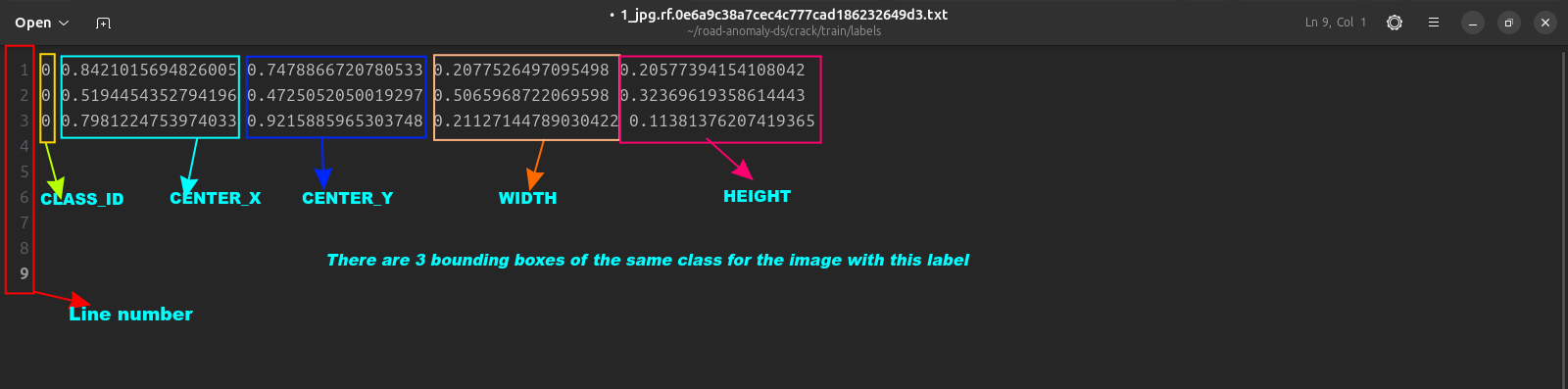
—————————————————————————————————————————————</strong></p>

<p><br />
We outline the objectives of this stage again. Which is to have a merged dataset with the three classes with label ‘0’ for pothole, ‘1’ for speedbump, and ‘2’ for crack. Also, this merged dataset is to have a 70-15-15 split for training, validation, and test sets respectively.</p>

<p>Here is how we achieve this:</p>
<ul>
  <li>We move all images in the train, val or test sub-folders of each datasets into a single folder say images. We do the same for the label files too.</li>
  <li>We check the data.yaml file in each class folder to understand the structure</li>
  <li>We remove unwanted labels and their ids if any by checking the data.yaml of each datasets</li>
  <li>We re-map label ids such as ‘0’ for pothole, ‘1’ for speedbump, and ‘2’ for crack</li>
  <li>We combine all images and labels from the three classes into a ‘images’ and ‘labels’ folder</li>
  <li>We split into the training, val, and test sets</li>
  <li>We create and update data.yaml file to correctly point to each sets and class.</li>
</ul>

<p>Note that we specially treat crack dataset as it is in segmentation format and not bounding boxes as object detection with YOLO requires. Here is <a href="https://machinesight.github.io">complete code</a> for this crucial step.</p>

<h3> Model Training </h3>

<p>
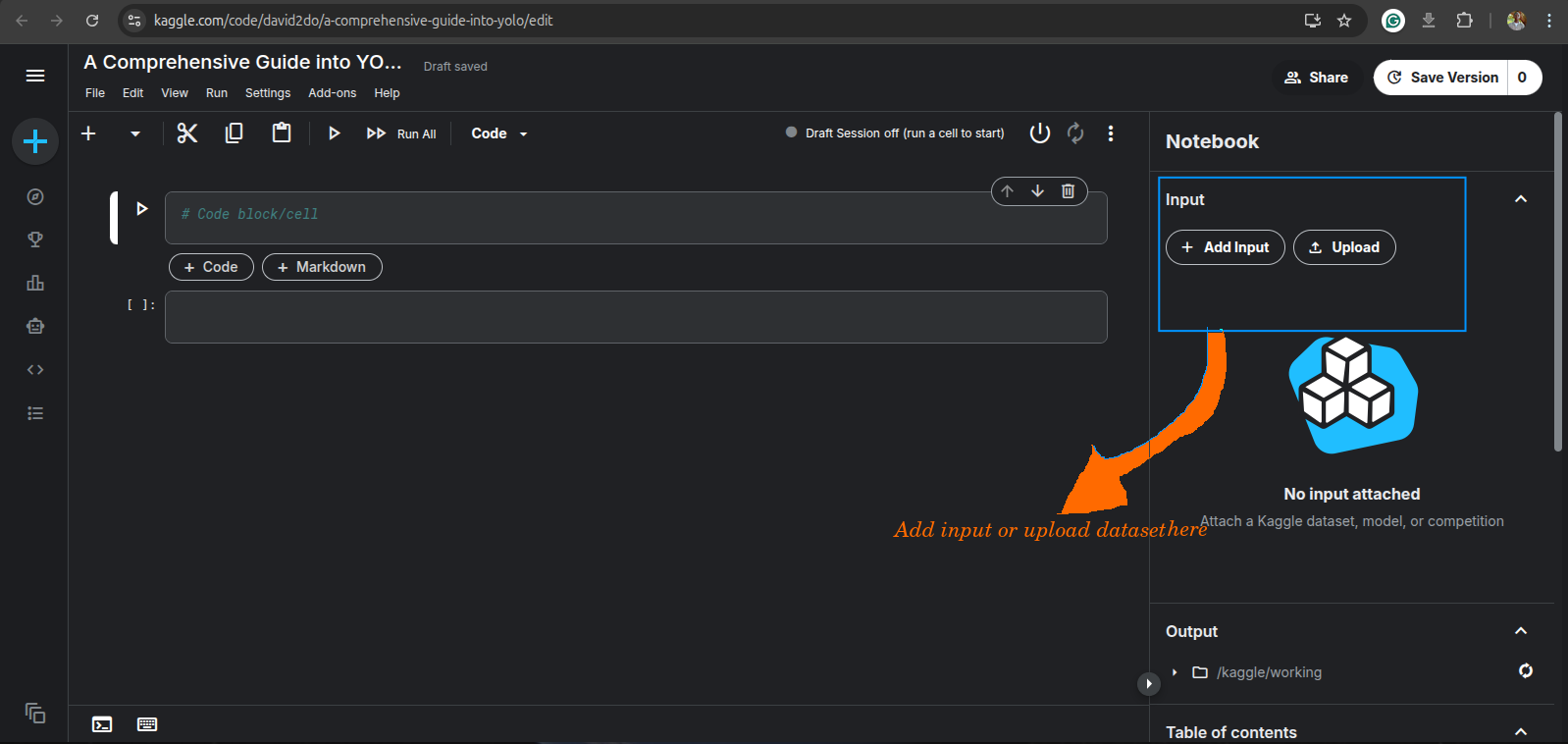
Here comes the fun part of model training. First, we create a new notebook with the kaggle account opened earlier, and upload the dataset or simply add it if you hadn’t gone through the dataset cleaning process, by searching for “<em>road_anomaly_ds</em>”, and adding it as input.</p>

<p><img src="/assets/images/2026-04-25/add-dataset.png" alt="Add or upload dataset to kaggle" /></p>
<figcaption>
 Add input or upload dataset to kaggle.
</figcaption>

<p><br />
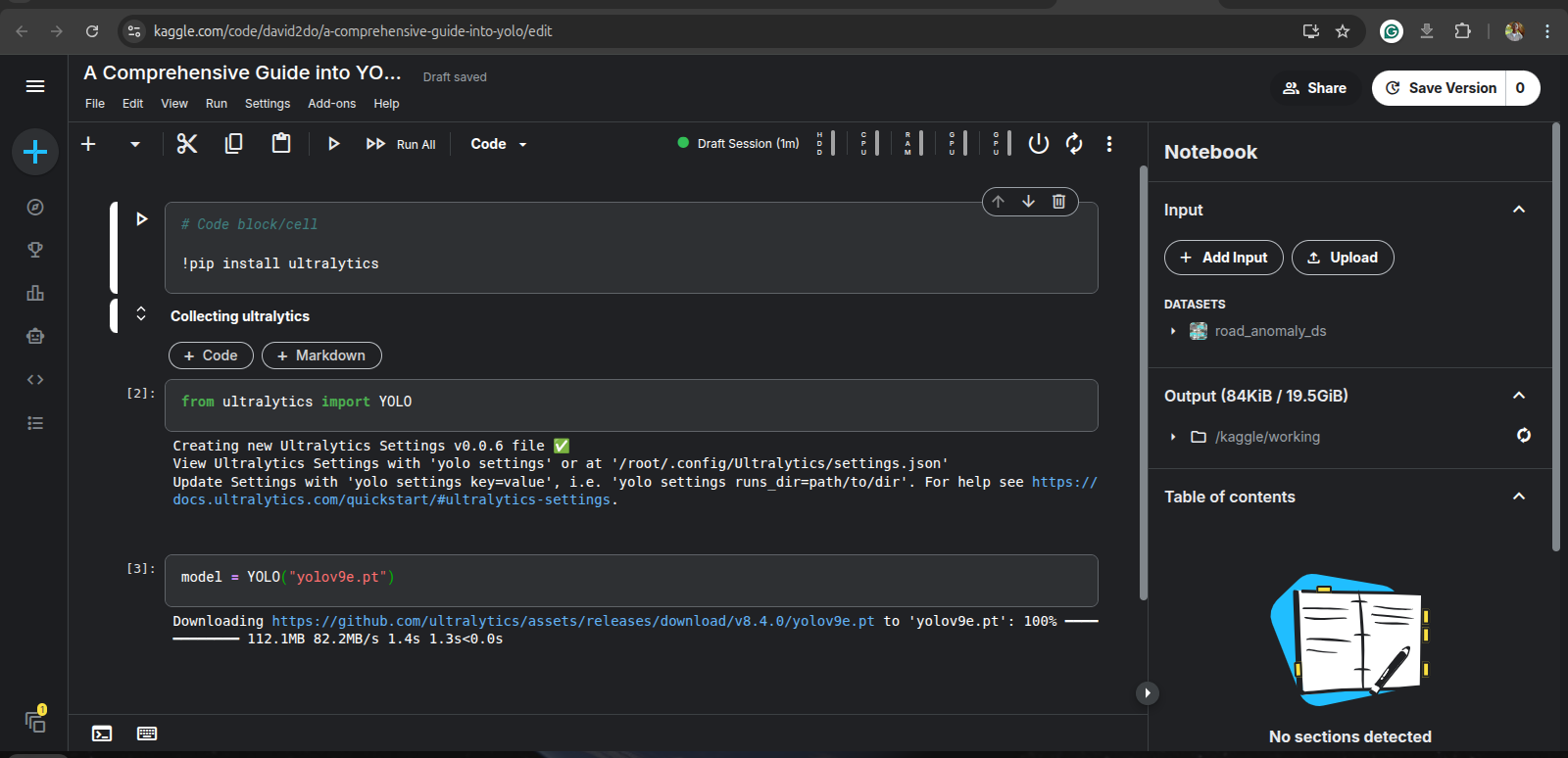
Then, we install the ultralytics package by running:</p>

<p><code class="language-plaintext highlighter-rouge">!pip install ultralytics</code></p>

<p>The ultralytics package provides a unified framework for training, validating and deploying AI models across platforms.</p>

<p>Once ultralytics is installed, import the YOLO module by running this code in a new cell:</p>

<p><code class="language-plaintext highlighter-rouge">from ultralytics import YOLO</code></p>

<p>For this tutorial, we will be training a yolov9e version on the dataset. Therefore, we instantiate YOLO with this version. Run:</p>

<p><code class="language-plaintext highlighter-rouge">model = YOLO("yolov9e.pt")</code></p>

<p>This will cause the model architecture and the COCO-pretrained weights to be downloaded on the kaggle session.</p>

<p><img src="/assets/images/2026-04-25/kaggle-progress.png" alt="Running codes on kaggle" /></p>

<p><br />
We train on our dataset:</p>
<div class="language-plaintext highlighter-rouge"><div class="highlight"><pre class="highlight"><code>model.train(
            data='/kaggle/input/datasets/david2do/road-anomaly-ds/data.yaml',
            epochs=100,
            batch=16,
            lr0=0.0001,
            imgsz=640,
            optimizer='AdamW',
            workers=8,
            project='/kaggle/working/runs',
            name='yolov9_lr_0.0001',
            mosaic=1.0,
            mixup=0.5,
            cutmix=0.5
           )
</code></pre></div></div>

<ul>
  <li>data: This is the path to the YAML file which points to the train, val and test set. It also contains the classes, and their labels</li>
  <li>epochs: Simply, the number of times the model learns from the train dataset. Selected as 100 here.</li>
  <li>batch: The number of samples the model sees before it “learns” (update it’s weights).</li>
  <li>imgsz: Input size for the images</li>
  <li>lr0: The learning rate; a key hyperparameter to experiment with.</li>
  <li>optimizer: An algorithm that updates the weight of the network. AdamW is used here.</li>
  <li>project and name: This is the path to save training results and files.</li>
  <li>mosaic, mixup, and cutmix: These are dataset augmentation techniques.</li>
</ul>

<p>
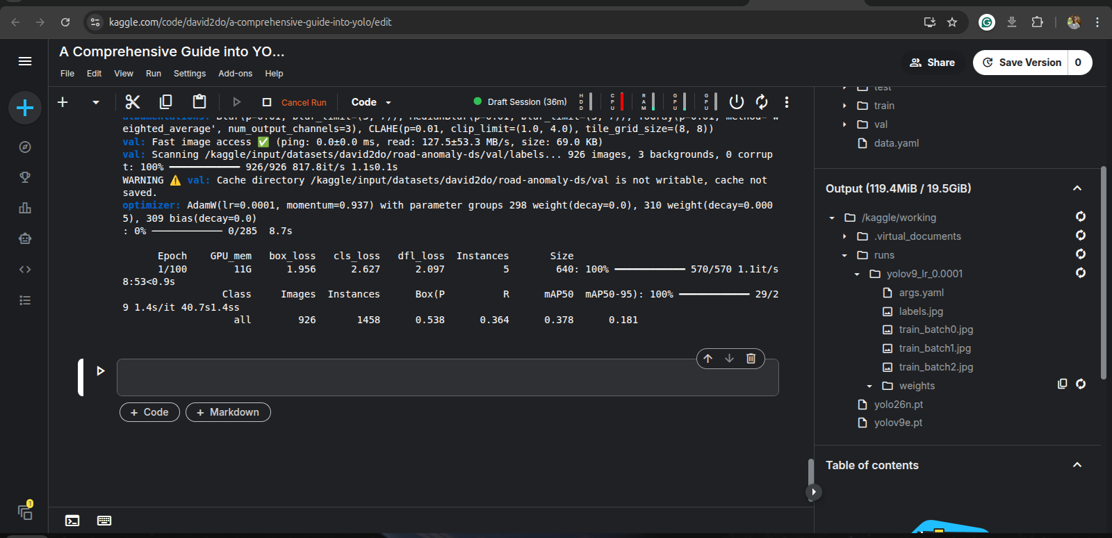
Running the code above may take significant time even with the use of GPU. Thus, it is suggested that you commit the notebook in kaggle so that it keeps running in the background even with the browser closed.
Once the training finishes, you can obtain the metrics at each epoch, like loss, precision, recall, mAP@50, mAP@50-95, and the model weights from the output if you commit the notebook, or at <code class="language-plaintext highlighter-rouge">/kaggle/working/runs/yolov9_lr_0.0001</code>. Ensure to download the content of <code class="language-plaintext highlighter-rouge">/kaggle/working/runs/yolov9_lr_0.0001</code> else, it will be lost when the session is stopped.</p>

<p>The model weights is found in the weights folder and there are two files: best.pt and last.pt. best.pt is the model weights when the highest mAP@50 occurred, while last.pt is simply the model weights at the last epoch.</p>

<p><img src="/assets/images/2026-04-25/epoch-1.png" /></p>
<figcaption>
 Training at epoch 1. The weights folder is found at the lower-right side.
</figcaption>
<p><br /></p>

<h3> Performance Evaluation and Testing </h3>

<p>
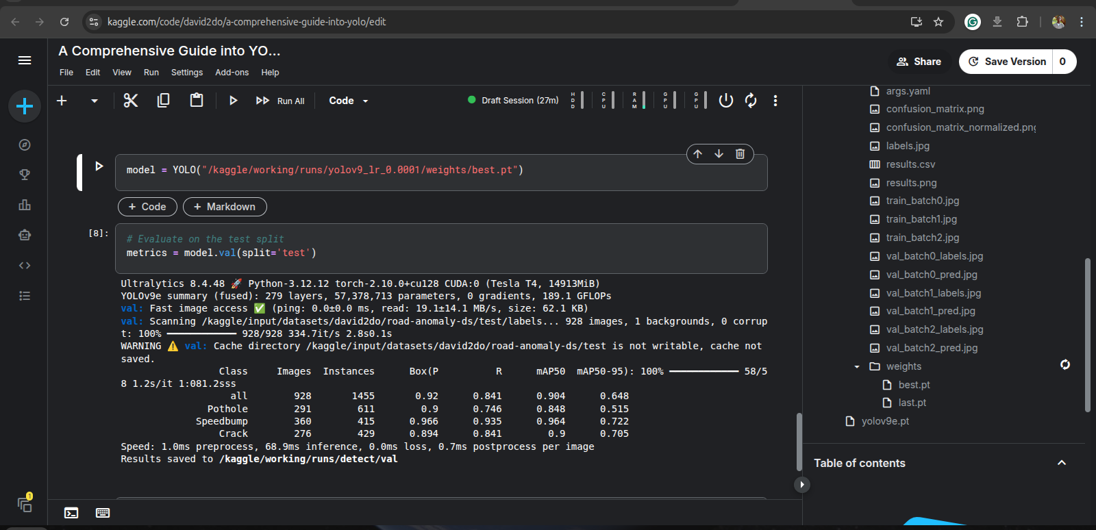
In this stage, we assess the performance of the model which we have trained. Though, we have via training, gotten performance metrics, it is however important (also a standard in ML) to evaluate the model on the test set of our dataset. It is recommended to use best.pt for this; we need to run this code:</p>

<div class="language-plaintext highlighter-rouge"><div class="highlight"><pre class="highlight"><code>model = YOLO("path/to/best.pt")
# Evaluate on the test split
metrics = model.val(split='test')
</code></pre></div></div>

<p>Executing the code above will use the test set to evaluate the overall performance of the model, from where we get the final performance metrics.</p>

<p><img src="/assets/images/2026-04-25/overall-performance.png" alt="YOLO performance on test set" /></p>
<figcaption>
 Performance evaluation carried out on the test set.
</figcaption>
<p><br /></p>

<p>And, that’s it! You now know how to build a model applicable in the real-world, whose output of detecting road anomalies can lead to complex decisions to enable an autonomous vehicle to for instance, slow, steer, or stop it.</p>

<p><b><em>Check out this kaggle <a href="https://www.kaggle.com/code/david2do/a-comprehensive-guide-into-yolo" target="_blank">notebook</a> for the training and performance source codes.</em></b></p>]]></content><author><name></name></author><summary type="html"><![CDATA[Training a YOLO model for object detection has been easy with ultralytics. This post gives a detailed overview of training a YOLO model for object detection right from custom dataset preparation to model evaluation and testing.]]></summary></entry><entry><title type="html">CNN Model Explainability with Grad-CAM</title><link href="machinesight.github.io/posts/cnn-model-explainability-with-grad-cam" rel="alternate" type="text/html" title="CNN Model Explainability with Grad-CAM" /><published>2026-02-22T21:57:30+00:00</published><updated>2026-02-22T21:57:30+00:00</updated><id>machinesight.github.io/posts/cnn-model-explainability-with-grad-cam</id><content type="html" xml:base="machinesight.github.io/posts/cnn-model-explainability-with-grad-cam"><![CDATA[<p><img src="/assets/images/2026-02-22/intro-img.jpg" alt="Object localization from image classification" /></p>

<p><br />
Deep learning models have become vital to the field of Computer Vision, and Artificial Intelligence. They have become the workhorse of modern machine learning algorithms. From image classification to image captioning, deep learning has been viewed as the most viable option.</p>

<p>However, how and why these models make predictions is a subject of on-going research. As a matter of fact, little is known about why a model correctly infers a dog as a dog; essentially, the ‘why’ they work is significantly obscure. Therefore, they are often treated as a black box, a cryptic tool of wonder.</p>

<p>Model explainability or eXplainable AI (XAI) aims to provide a clear understanding of what led to a prediction through visual explanation. In this post, we introduce a notebook that use Gradient-weighted Class Activation Mapping (Grad-CAM) to implement model explainability in CNN for image classification with tensorflow. We then finally segmented the part crucial for the classification (a form of object localization).</p>

<p><strong>The background:</strong> After training a well-performing image classifier for medical diagnostics with a post-graduate researcher, the need arose to see that the model really is considering the aspect of the image necessary for accurate prediction. It was pleasing to realize the model works correctly after obtaining the Grad-CAM. So, if you have been wondering what your DL model “looks” at to classify an image, then the notebook is for you.</p>

<p>Access the notebook <a href="https://www.kaggle.com/code/david2do/cnn-model-explainability-with-grad-cam">here</a>. I hope you enjoyed it.</p>

<p><em>Kindly note that this post will be updated later for analysis and detail.</em></p>]]></content><author><name></name></author><summary type="html"><![CDATA[This post examines how Grad-CAM can be used to explain CNN model predictions, focusing on visualizing attention maps.]]></summary></entry><entry><title type="html">What Images Really Are: Considering Images As Computational Representations</title><link href="machinesight.github.io/posts/what-images-really-are" rel="alternate" type="text/html" title="What Images Really Are: Considering Images As Computational Representations" /><published>2026-01-24T11:30:55+00:00</published><updated>2026-01-24T11:30:55+00:00</updated><id>machinesight.github.io/posts/what-images-really-are</id><content type="html" xml:base="machinesight.github.io/posts/what-images-really-are"><![CDATA[<p><img src="/assets/images/matrix_style.webp" alt="Matrix-like Computer Screen" /></p>
<figcaption>
  Binary code background. Source: <a href="https://www.freepik.com/free-photo/binary-code-background_1182031.htm">Freepik</a>
</figcaption>

<p><br />
The digital world is one of the most fascinating wonders of human creation. Just as the universe is governed by natural laws established by God, the digital world is entirely defined and yet controlled by man. To better interact with our surroundings, we need sight; spatial data from the eyes interpreted by the brain. We, therefore, desire a representation of our visual surroundings to create a twin in the digital world. These representations are called Images.</p>

<p>In this blog post, we will examine images from the standpoint of a computer, and not the camera. (Picture it as what we “see” in the brain and not the eyes). Therefore, little will be said about their formation or geometry.</p>

<p>Images are organized collection of numbers called pixels. Images being numbers is unsurprising as computers understand only numbers. A pixel is a number or list of numbers typically grouped in three or four sets as we will better describe later when we look at types of images. These pixels serve as atoms; the building blocks for any image. The higher the number of pixels in an image, the better the quality or resolution.</p>

<p>Think of pixels as pebbles on a shore. They can easily be arranged to form different shapes based on their size or color. The smaller they are, the more detailed the shape formed is. Likewise the smaller a pixel is, meaning it gives room for other pixels, the greater the representation and consequently, the better the image looks. We see that our understanding of pixels is invariably the understanding of images.</p>

<p>Since an image is a matrix, it is represented with rows and columns; where the number of rows specify the height, and the number of columns is the width.  Hence, the dimension of an image is usually in the form: (rows, columns). For example, the image below has 1920 pixels along its height and 2560 pixels across its width. The upper left corner is the origin of the image coordinate system by convention, and indexing starts from zero.</p>

<figure>
  <img src="/assets/images/image_coordinate.png" alt="Image coordinates system" />
</figure>

<p>There are two major types of images:</p>

<p><strong>Grayscale Images</strong>:- In this representation, pixels take a single value which are either black or white or any shade in between. For uint8 (8-bit unsigned integer) which is most common, 256 values (2^8) are used. These values range from 0 to 255. 0 represents complete black, 255 for white, and numbers in-between for different shades of gray. We therefore see that these values encode the intensity of the pixel. The figure below is a comprehensive insight into this.</p>

<figure style="text-align: center;">
  <img src="/assets/images/grayscale_example.png" alt="Grayscale image with pixel values" />
  <figcaption>Grayscale image of hand-written 3 on the left with pixel values on the right. Source: MNIST dataset</figcaption>
</figure>

<p>Note that “Black and White” images are simply stripped-down versions of grayscale images. Here, the pixel values are either black or white; hence its’ name. The pixel has values of either 0 (black) or 1 (white). For this reason, they are also referred to as binary images.</p>

<p><strong>Color Images</strong>:- Most images we interact with belongs to this. Instead of a single value, a pixel is encoded as a set of three numbers. Each number correspond to a channel in a color space. A color space is simply a specific organization of colors that typically represents all possible human-perceivable colors. One of the most common color spaces is the RGB color space, which contains Red, Green, and Blue channels.
Like grayscale, the R, G and B channels also range from 0 to 255 using uint8. These values also mean the intensity of the color elements.</p>

<p>In RGB, white is represented as (255, 255, 255) and black as (0, 0, 0). Other colors are a variation/combination of these three numbers. We see that this representation yields about 16 millon unique colors, many of whom the human eyes cannot perceive. The demonstration below is a thorough low-level understanding of this.</p>

<figure style="text-align: center;">
    <p align="center">
        <img src="/assets/images/zoomed_in_pixels.gif" alt="Zoom-in to pixel-level GIF" />
        <figcaption>Zooming into the pixel level of RGB color image</figcaption>
    </p>
</figure>

<p>Other notable color space is HSV (Hue, Saturation and Value) which is crucial in computer vision for performing image analysis. Chances are that your image displaying software uses RGB than HSV.</p>

<p>As a special case, PNG images support a 4th channel called the “alpha” channel. The alpha channel contains transparency information, allowing specific regions within an image to appear transparent. Graphics and artistic design is one area of usage for PNG images.</p>

<p>One might ask, how then are videos represented? The answer to that seems clear. Just take a series of images, join them in a sequence, and play them in a loop (of a specified speed); then you have a video! The images in a video are called frames.</p>

<p>Thanks for coming to the end of this writing. I believe by now, you not only see an image for what it is. But you could see the numbers behind the scenes beautifully arranged in rows and columns, literally. (Oops, you are now a Terminator!).</p>]]></content><author><name></name></author><summary type="html"><![CDATA[This post examines what images really are, delving into pixel-level representation, and how they can be used in computer vision tasks.]]></summary></entry></feed>